A gentle introduction to VRP problem

VRP stands for Vehicle Routing Problem. It has attracted a great deal of interest from companies over the past two decades because the study of this problem makes it possible to understand the impact of logistics on business and to optimize it.

The first time VRP appears is in a paper published in 1959, written by George Dantzig and John Ramsen and applied to a gas delivery. It is a generalization of the TSP problem.

VRP answers the following question: What are the optimal routes for a fleet of vehicles to meet the demand of a set of customers?

VRPs belongs to NP-HARD problem, because finding the optimal solution require a lot of effort and time.

So in the real scenario heuristics or metaheuristics are used to obtain solution.

VRP variants

In literature there are a lot of different classification of VRP [1]. Here a list of the commons VRP problem. Notice that each class of VRP has different constraints and specialize a particular aspect of the problem.

• CVRP or Capacitated VRP, HFVRP (Heterogeneous VRP)
• OVRP or Open VRP
• 2D-VRP or 3D-VRP
• VRPSF or VRP Satellite facilities
• TTVRP or Truck and Trailer VRP
• ConsVRP or consistent VRP
• VRPTW or VRP with time windows, VRP with soft time windows
• TSPTW -> TSP with time windows.
• DVRP or Dynamic VRP
• GVRP or Green VRP, PRP or Pollution routing problem, EVRP o Electric VRP, HVRP or Hybrid VRP
• SVRP or Stochastic VRP
• MDVRP or Multi Depot VRP, Collaborative VRP
• SDVRP or Split Delivery VRP
• PVRP or Periodic VRP
• RVRP or Rich VRP
• PCTSP ,Price collecting TSP
• PCTSPTW , Price collecting TSP with Time Windows

VRP math formulation

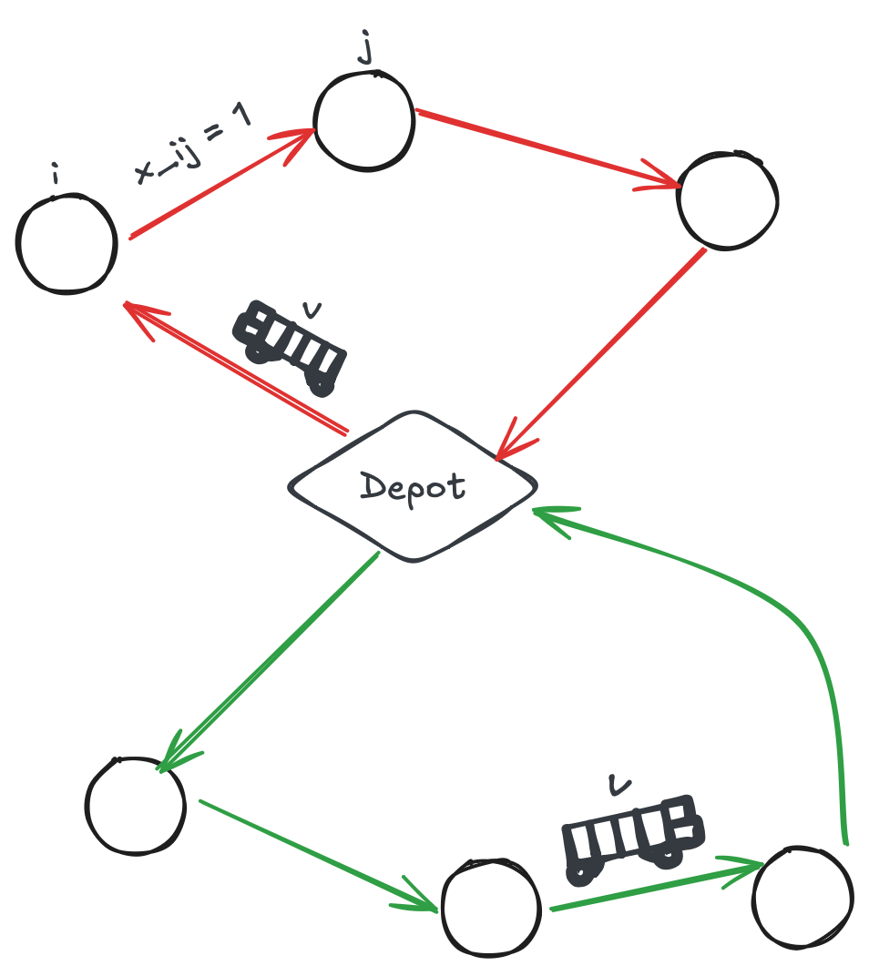Figure 1. CVRP Image Example. The nodes are the customers and in the center there is the single depot.

A Capacited Vehicle Routing Problem can be described the following manner. Consider the problem with a single repository. The nodes represent the customers C={1,2,…,n} with which some demand ki is associated. The vehicles leaving and returning to the depot belong to the set V={1,2,…,m}. In this case the vehicles are homogeneous, so they will have the same carrying capacity qi. If there is an arc connecting node i to node j due to vehicles v∈V then the variable xijv will have value 1. Each arc will have a weight corresponding to the distance from node i to node j represented by dij.

The goal is to minimize the total distance of the route, subjected to different constraints:

• Flow constraint

  The number of vehicles entering a node must equal the number of vehicles leaving the node.

• Each node (customer) must be visited once

• Every vehicle leaves the depot

  Note that the index i=1 since it is the deposit while the index j=2

• Capacity constraint

  Each vehicle has a certain possible amount that it can carry. So it is necessary not to exceed that threshold , considering that in the treated problem all vehicles have the same capacity (homogeneous vehicle fleet).

References

1. 1. Elatar S, Abouelmehdi K, Riffi ME: The vehicle routing problem in the last decade: variants, taxonomy and metaheuristics. Procedia Computer Science 2023, 220:398–404.

Published by Samuele Simone, PhD Student in VRP and AI @UNIMI